
Abyssal Mixing at the Equator
Abyssal mixing near the equator: A microstructure turbulence study
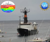
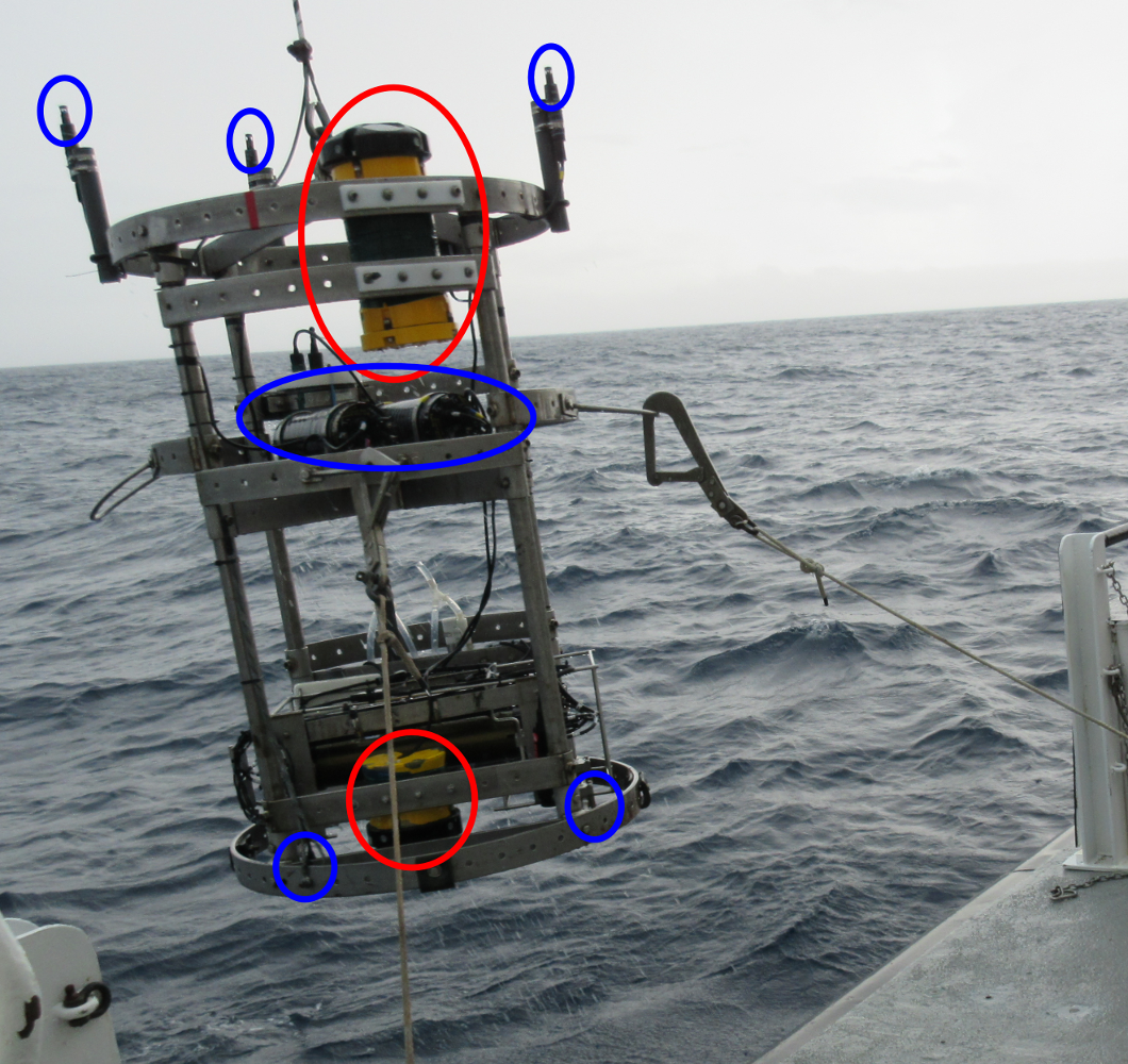
In December 2014 I was invited to participate in a five-week research cruise to the equatorial Pacific by Professor Jim Moum. Jim is a world leader in making observations of small-scale turbulent mixing using a number of cutting-edge microstructure turbulence instruments developed by his group at Oregon State University. The research cruise aboard the R/V Oceanus (Figure 1) was aimed at measuring turbulence both in the upper ocean on the equator, but also at testing a new instrument for making measurements of mixing in the abyssal ocean. The abyssal measurements were made using a CTD Chi-pod instrument (see Fig. 2) that measures temperature variability at very high frequency as the instrument is lowered into the deep ocean.
Strong abyssal mixing over smooth topography!
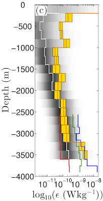
Mixing in the abyssal oceans is generally thought to occur mostly above rough seafloor topography such as seamounts and the mid-ocean ridges. Here, tidal and geostrophic currents flow over the topography generating internal waves which break and mix the fluid. This picture has been developed over the last several decades through extensive microstructure turbulence field campaigns. Much of this data was recently compiled into a single data set by Waterhouse et. al. (2014), who showed that indeed mixing measurements over rough topography and mid-ocean ridges showed turbulent mixing intensities, quantified with the turbulent kinetic energy dissipation epsilon, an order of magnitude larger than those over smooth topography (compare red, green and blue curves in Fig. 3).
Our cruise in December 2015 was to a region near the equator where the seafloor was particularly flat and smooth compared with the global average. Thus we were surprised to find very energetic mixing, with energy dissipation rates just as strong as that found elsewhere over mid-ocean ridges within the bottom 700m of the ocean (compare orange line with blue line in Fig. 3 below 3200m). What was going on? Was there something special about the equator?
Where does the energy come from?
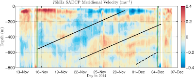
If the energy that drives this mixing is not coming from the seafloor through flow interactions with rough topography, then it must come from the surface. One possibility is the downwards radiation of low-frequency equatorial waves. These waves are commonly found in the surface equatorial oceans and are generated by wind forcing and instabilities (such as tropical instability waves). While we did not have any temporal measurements to investigate the existance of waves in the deep ocean (each profile of the CTD Chipod represents just one point in time), we did have a long-time series of velocity measurements in the upper 800m made by the shipboard ADCP instrument (Fig. 4). These measurements did indeed show evidence of a low-frequency wave (upward propagating phases highlighted with black lines in Fig. 4). In fact, the properties of the measured wave were consistent with the dispersion relation for a downward propagating equatorial Yanai wave with downward energy flux ~2mWm-2. This downward propagating wave had sufficient energy flux to drive the abyssal mixing estimated from the Chipod instrument to average ~1mWm-2.
Non-traditional wave trapping
The downward propagating equatorial Yanai wave may have sufficient energy to drive the mixing, but the remaining question is why would it break and drive mixing in the bottom 700m? Wave breaking typically occurs at critical layers created by a background mean flow, or where the vertical wavelength of the wave becomes small in regions of high stratification. However, we did not observe any mean flows, and the stratification generally reduces towards the seafloor. One possibility, normally neglected in most oceanograhic studies, is the influence of the horizontal component of Earth’s rotation (the so called non-traditional effects). The dispersion relation for a classical internal waves is,
where is the wave frequency, f is the Coriolis parameter,
is the stratification and
is the slope of wave characteristics. Since all terms in this equation are positive, this implies that a wave can only exist equatorward of where its frequency omega is equal to f (since f reduces towards the equator). This results in the wave being trapped within its so-called ‘inertial latitudes’ (thick lines in Fig. 5a). However, when the non-traditional terms are included, the dispersion relation acquires an extra term.
The additional term, dependent on the horizontal component of Earth’s rotation , can be negative and allows wave to exist poleward of their inertial latitude in regions where the stratification is small, i.e. near the seafloor. Practically, this creates trapping regions near the seafloor where wave energy can enter but cannot leave, and thus builds up and breaks driving mixing (compare inverse Richardson number between traditional and non-traditional cases in Fig. 5). Thus these non-traditional effects may be responsible for the trapping of the energy of the downward propagating equatorial Yanai wave, resulting in the bottom-intensified mixing over smooth topography that we observed with the Chipod.
For more information please see my article published in Geophysical Research Letters (Evidence for Seafloor-Intensified Mixing by Surface-Generated Equatorial Waves) or feel free to contact me. This article was also the subject of several media releases that are also worth a look:
Environmental Monitor: Study Of Deep Turbulence Reveals Ocean Currents Insights